
Nori ↑
Introduction ↑
Building upon the Nori renderer from ETH Zurich's Computer Graphics course (FS2025), Nori represents my exploration into advanced rendering techniques. Here I document the features I implemented beyond the course requirements, along with my notes and validations.
Table of Contents
Emitters ↑
Spot Light ↑
Spotlights emit light in a cone of directions from their position. This is discussed in chapter 12.2.1 of the PBR book.
Description ↑
Files created or modified:
src/spotlight.cpp
Validation scenes:
scenes/nori-beyond/spotlight/cbox.xmlscenes/nori-beyond/spotlight/cbox_mitsuba.xml
A new emitter type SpotLight is implemented in the file spotlight.cpp.
The origin of the light is at , and points towards the axis. A spot light is defined by two angles -- falloffStart, where everything inside this angle is fully illuminated (intensity multiplier = 1), and totalWidth, where illumination fades to black at this angle, and everything outside is dark (intensity multiplier = 0). To avoid expensive operations, I store the the cosines of the angles cosFalloffStart and cosTotalWidth, and since decreases as increases, . To create a soft transition zone (penumbra) in the outer cone, I use the SmoothStep function, which is a cubic function (Hermite interpolation), that takes in , where is the cosine angle between and the vector with direction pointing from the light origin to the point in scene:
- Compute and if or .
- Return (Hermite interpolation)
The angular intensity is the radiant intensity in the direction (power emitted per solid angle in direction ), and is given by
A surface patch at point subtends a small solid angle around direction , with the relation , where is the angle between the surface normal at and direction from to the light. The power arriving at from that infinitesimal solid angle is given by
The irradiance on the patch is . The radiance is defined so that
Derivation of flux (not used explicitly in this implementation because of the uniform sampling strategy)
A spherical cap (cone of half-angle ) has solid angle . Within the region of falloffStart, intensity is constant, so flux in that region is
Between falloffStart and totalWidth, the intensity decreases smoothly to 0. The PBR book approximates the integral by assuming that intensity in the region averages to half the peak value. The solid angle of the penumbra annulus is . If the average intensity is , then
Total flux is thus
SpotLight::eval(...)
Delta emitters have zero area so there is measure-zero probability of hitting them via BSDF sampling.
SpotLight::sample(...)
First assign the fields of the emitter query record lRec given the position of the light and the reference point . Then compute the angle attenuation term using given the cosine of the angle between the m_direction (direction of spot light) and the vector pointing from the light to (lRec.ref). Finally compute the intensity and return the radiance.
SpotLight::pdf(...)
Delta lights have zero measure, thus PDF = 0. This is required for MIS.
Spotlight::samplePhoton(...)
First sample a direction from the light using squareToUniformSphereCap and assign the sampled direction to ray. Then compute the angle attenuation term using given the cosine of the angle between the m_direction (direction of spot light) and the sampled direction. Finally return the photon power, which is the intensity divided by the sampling PDF.
Validation ↑
I compared my implementation with Mitsuba with the Cornell box scene with two cubes, and a spot light positioned behind the right one, pointing towards the left one.
I also updated path_mis.cpp to support delta lights (spotlights and point lights) by modifying the MIS weight calculation. For delta lights (detected by checking if ems_lRec.n.isZero()), I set the MIS weight to 1.0 since delta lights cannot be sampled by BSDF sampling (the probability of randomly hitting a point light via BSDF is zero). This ensures that only emitter sampling contributes when rendering scenes with delta lights, preventing the image from being incorrectly darkened by MIS weighting.
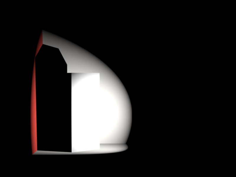
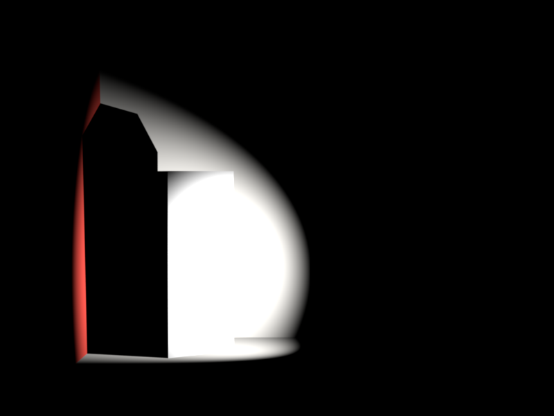
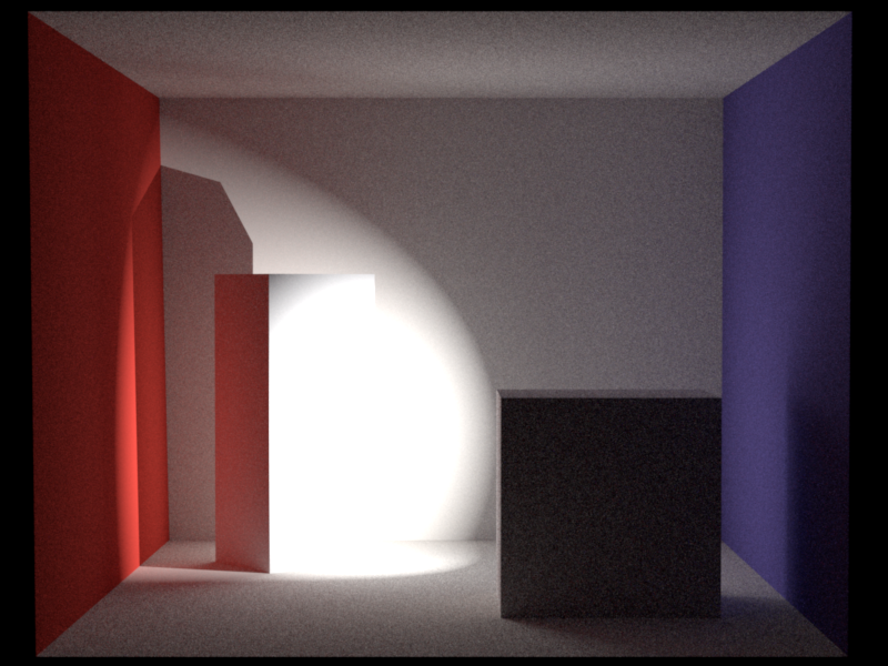
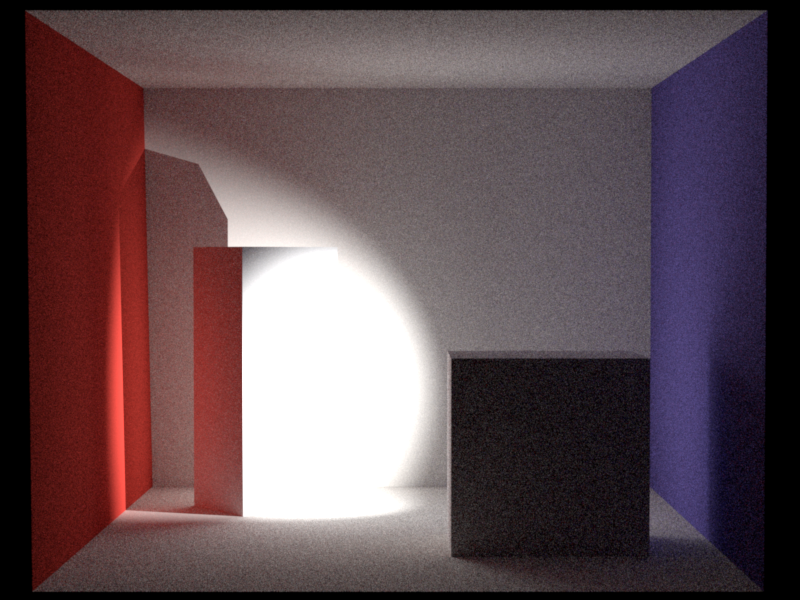
There is a reasonable difference in rendered images. In my implementation, after computing , I apply a Hermite interpolation (SmoothStep) following the PBR book, which creates an "S-curve" falloff. My spotlight hence stays brighter for longer near the center (the "shoulder" of the S-curve) and fade out more gradually near the absolute edge (the "toe" of the S-curve) compared to Mitsuba's sharp linear drop, which applies applies a pure linear ram. Also, my interpolation domain is cosine where Mitsuba is the angle itself. I believe that the visual differences make sense based on these two implementation differences.
Directional Light ↑
Directional Light is also known as distant light, which desccribes an emitter that deposits illumination from the same direction at every point in space. This feature is discussed in chapter 12.3 of the PBR book.
Description ↑
Files created or modified:
src/directionallight.cpp
Validation scenes:
scenes/nori-beyond/directional_light/
A new emitter type DirectionalLight is implemented in the file directionallight.cpp.
The radiance at a point from direction due to directional light with direction is given by
The physical reason that directional lights make sense is that for point lights, where is the distance from the point light. For directional lights, . However, the emitting area also grows as . The two effects cancel.
DirectionalLight::eval(...)
Delta emitters have zero area so there is measure-zero probability of hitting them via BSDF sampling.
DirectionalLight::sample(...)
Given a shading point , we sample the incoming direction deterministically since there is only one valid direction. We set:
- (toward the light source)
- (a fictitious point far away)
- (delta distribution, handled specially)
- Shadow ray from toward with infinite extent
The returned radiance is simply . Unlike area lights, there is no falloff since the light is infinitely distant.
DirectionalLight::pdf(...)
Delta lights have zero measure, thus PDF = 0. This is required for MIS to correctly handle the delta distribution---the MIS weight computation uses this PDF, and returning 0 ensures that BSDF-sampled paths that happen to align with the light direction don't incorrectly contribute.
DirectionalLight::samplePhoton(...)
For photon mapping, we need to emit photons that cover the entire scene uniformly from the light direction. Following PBR book 12.5, we:
- Sample a point on a disk of radius perpendicular to the light direction
- Position this disk behind the scene (offset by along )
- Emit a ray from this point in direction
The disk sampling uses an orthonormal frame built from :
where is a uniform disk sample and form an orthonormal basis.
The photon power is (radiance times the disk area), which accounts for the uniform PDF of over the sampling disk.
Validation ↑
Environment Map Emitter ↑
An environment map emitter (infinite area light) wraps the scene in an infinitely large sphere textured with an HDR image, so that every direction in space receives radiance defined by the map. This is discussed in chapter 12.4 of the PBR book.
Description ↑
Files created or modified:
src/envmap.cppinclude/nori/emitter.hinclude/nori/scene.handsrc/scene.cpp- All integrators:
src/path_mis.cpp,src/path_mats.cpp,src/path_ris.cpp,src/direct_mis.cpp,src/direct_mats.cpp,src/direct_ems.cpp,src/direct.cpp envmap_sampling_viz.pylatlong_to_equalarea.py
Validation scenes:
scenes/nori-beyond/environment_map/cbox_envmap.xml
A new emitter type EnvironmentMap is implemented in the file envmap.cpp, registered as "envmap".
For every direction in the sphere, light comes from that direction with some radiance . If we shoot a ray and it misses everything in the scene, we look up the ray direction in the HDR environment image. However, since our HDR file is a 2D image, but directions live on a sphere, we need a mapping
Following Chapter 3.8.3 in the PBR book, the environment map image uses the equal-area octahedral parameterization rather than the traditional equirectangular (latitude-longitude) projection. The traditional equirectangular mapping compresses solid angles near the poles (), so polar pixels cover vanishingly small solid angles. This requires an explicit correction in the sampling distribution and introduces a Jacobian that becomes singular at the poles.
The equal-area octahedral mapping avoids these issues. It combines:
- Octahedral projection: Project the unit sphere onto the faces of an octahedron, then unfold the octahedron into a square
- Concentric disk-to-hemisphere mapping: Apply an area-preserving mapping (from Shirley & Chiu 1997) so that each pixel subtends exactly the same solid angle:
Forward mapping (sphere to square, implemented in src/envmap.cpp as a helper function equalAreaSphereToSquare(const Vector3f &d)): Given a direction on the unit sphere, the mapping computes . The setup is as follows: Imagine an octahedron inscribed in a sphere. The ocatahedron can be unfolded to a square -- the top four faces of it (where ) map directly to a diamond in the center of the 2D square, and the bottom four faces (where ) are "folded out" into the four corner triangles.
- In the setup described above, we can then define the radius from latitude. The latitude (circle on the sphere at a specific height ) is mapped to the square such that the point on the square sits on a concentric diamond around the origin if or a concentric corner triangle near if . This is defined by , which means that:
- when , the radius on the square is given by
- when , the radius on the square is given by
- Next we determine where along that line the point lands. We first work in the positive quadrant of using and . Let
Then we approximate using a minimax polynomial. In implementation, the exact coefficients in Nori are taken from PBRT's source code, indouble a = max(fabs(x), fabs(y)); double b = min(fabs(x), fabs(y)); b = (a == 0) ? 0 : b / a;src/pbrt/util/math.cppinsideEqualAreaSphereToSquare(), where the authors mention that the code is "Via source code from Clarberg: Fast Equal-Area Mapping of the (Hemi)Sphere using SIMD". This avoids callingatan()directly:
This gives a normalized position along the diamond edge in the positive quadrant. The corresponding coordinates aredouble phi = P(b); // approximates (4/pi) * atan(b) if (fabs(x) < fabs(y)) phi = 1 - phi;
For the upper hemisphere (), this already lies on the inner diamond . For the lower hemisphere (), the point must be folded out to the corner triangle:double vp = phi * R; double up = R - vp;
After this step, lies in the positive quadrant with the correct radius: for the upper hemisphere and for the lower hemisphere.if (z < 0) { swap(up, vp); up = 1 - up; vp = 1 - vp; } - We then restore the original and signs and remap from to :
This places the point in the correct quadrant of the final square.double u_signed = copysign(up, x); double v_signed = copysign(vp, y); double u = (u_signed + 1) / 2; double v = (v_signed + 1) / 2;
Inverse mapping (square to sphere, implemented in src/envmap.cpp as a helper function equalAreaSquareToSphere(const Point2f &p)): Given , we recover . Following PBRT, it uses a direct branch-free formula that maps the square back to the sphere.
-
Remap from to and work with in that signed square. Their absolute values determine how far the point is from the diagonal , which separates the upper and lower hemispheres:
double up = fabs(u');
double vp = fabs(v');
double signedDistance = 1 - (up + vp);
double r = 1 - fabs(signedDistance);
Here,
signedDistancedetermines the hemisphere: positive means upper hemisphere, negative means lower hemisphere. The quantity is the same equal-area radius used by the forward map. -
Reconstruct the angular parameter within the positive quadrant:
double phi = (r == 0 ? 1 : (vp - up) / r + 1) * (M_PI / 4);This is the inverse of the forward-map relation that used to split the radius into two square coordinates. It recovers the angle within one octahedral sector.
-
Convert back to a 3D direction:
double z = copysign(1 - r * r, signedDistance);
double cosPhi = copysign(cos(phi), u');
double sinPhi = copysign(sin(phi), v');
double rFactor = r * sqrt(2 - r * r);
return Vector3f(cosPhi * rFactor, sinPhi * rFactor, z);
These steps are not direct inverses of the
swap()/1 - ufolding logic used inequalAreaSphereToSquare(). Instead, they reconstruct the sphere point from the equal-area square parameterization in one shot:z = copysign(1 - r^2, signedDistance)recovers the hemisphere and height on the sphere.cosPhiandsinPhirecover the azimuthal direction inside the correct quadrant by attaching the signs of and .rFactor = r\sqrt{2-r^2}is the radius of the projected point in the -plane, coming from PBRT's equal-area disk-to-hemisphere mapping.
To find the light coming from direction , we convert that direction into map coordinates , find which pixel that lands on in our image, take that pixel's color and multiply it by a brightness scale:
Uniform sphere sampling would be very inefficient since most of the radiance is typically concentrated in a small region (e.g. the sun). Following PBRT Chapter 12.4, we build a 2D piecewise-constant distribution over the image pixels.
Because the equal-area mapping ensures every pixel covers the same solid angle, the sampling weights are simply the luminance of each pixel, and no correction is needed. This is one of the key advantages of the equal-area mapping.
The distribution is built in two levels:
- Conditional CDFs (per row): For each row , build a CDF over columns weighted by
- Marginal CDF (over rows): Build a CDF over rows weighted by the integral of each row
Sampling draws a row from the marginal CDF, then a column from that row's conditional CDF, both via binary search. The sampled pixel is converted back to a direction via EqualAreaSquareToSphere.
The PDF in solid-angle measure is obtained by a simple change of variables. Since the equal-area mapping has Jacobian (mapping to the unit sphere of area ):
where is the discrete probability density in image space.
include/nori/emitter.h
Two functions isEnvironment and evalEnvironment are added. isEnvironment returns true if this is an environment emitter and is false by default. EnvironmentMap::isEnvironment(...) overrides to true. evalEnvironment is needed for the case where a ray escapes the scene entirely. With no intersection information, we only have the ray's direction. evalEnvironment is a direction-only convenience method added to this base Emitter class for this specific case.
Scene::addChild(...)
In the header file, we add a single stored pointer to the environment light m_envEmitter and the method getEnvironmentEmitter that returns the pointer to the environment emitter.
In the case of an emitter, we additionally check if the emitter is an environment light and if pointer m_envEmitter is already non-null, i.e. the scene already has an environment emitter stored, in which case we throw an exception.
EnvironmentMap::eval(...)
Implements EnvironmentMap::evalEnvironment(...) with the direction lRec.wi. The evaluation proceeds in the following steps:
-
Transform the world-space direction on the unit sphere into 2D texture coordinates using
equalAreaSphereToSquare -
Convert the continuous coordinates to pixel space with pixel-centered addressing:
The offset treats pixel centers as integer coordinates.
-
Compute the integer coordinates of the four corners:
Compute the fractional offsets:
Clamp all coordinates to the valid range and respectively to handle boundary cases.
-
Fetch the four corner pixel values from
m_data:Blend using bilinear interpolation:
This provides smooth filtering across pixel boundaries, reducing aliasing compared to nearest-neighbor lookup.
buildDistribution()
This is a method that fills in EnvironmentMap's member variables m_marginalPdf, m_marginalCdf, m_conditionalPdf and m_conditionalCdf using m_width, m_height, m_data. m_conditionalCdf is an array of size m_height * (m_width + 1) since each row requires (m_width + 1) boundary points to define its m_width bins and there are m_height rows in total. m_marginalCdf is an array of size m_height + 1 for row sampling, according to a marginalWeights array.
It follows the steps:
- Build the conditional CDF for each row. For each row , compute the base (start of that row's CDF inside the flat
m_conditionalPdfarray) and initializem_conditionalPdf[base] = 0. - For each pixel in row , retrieve the luminance by looking up the pixel value in
m_data. Then build a prefix sum asnd store that intom_conditionalCdf[base + x + 1]. - The total brightness of the row is then stored in
m_conditionalCdf[base + m_width], which is then saved inmarginalWeights[y]to inform row sampling (brighter rows should be sampled more often). - If the row has non-zero brightness, normalize the row CDF so that it becomes a proper CDF in . We also fill in
m_conditionalPdfusing the luminance of each pixel in the row normalized by this row total. Otherwise, it means that the row is completely black, and to avoid division by zero, we fall back to uniform sampling, where each column of the row gets probability1 / m_width. - After building
m_conditionalCdfandm_conditionalPdf, we buildm_marginalCdfandm_marginalPdfusingmarginalWeights. Similar to the previous step, we normalizem_marginalCdfandm_marginalPdf.
buildDistribution is called once after the image data is loaded. The CDFs m_marginalCdf and m_conditionalCdf are then used to sample a pixel on the environment map, and m_marginalPdf and m_conditionalPdf are used to compute the Monte Carlo radiance of the sampled pixel.
EnvironmentMap::sample(...)
- Sample a row from the marginal CDF using the first random number and record
- Sample a column from that row's conditional CDF using the second random number and and record
- Convert the sampled pixel to the coordinates in a , then to a direction using
EqualAreaSquareToSphere - Compute the solid-angle PDF where
- Set
lRec.pto a distant point along (at ), and the shadow ray to - Return .
EnvironmentMap::pdf(...)
We convert the direction lRec.wi to image coordinates using EqualAreaSphereToSquare and then look up the marginal and conditional PDFs, and returns .
EnvironmentMap::samplePhoton(...)
For photon mapping, we sample a direction from the environment map's importance distribution, then place the photon origin on a disk of radius perpendicular to that direction (similar to the directional light approach). The photon power is .
Integrator Modifications
The environment map is a non-geometric emitter so rayIntersect can never find it. Two changes were needed in every integrator:
- Camera rays that miss geometry: Instead of returning black, check for an environment emitter and return . This renders the environment as the background.
- BSDF-sampled rays that escape the scene: Evaluate the environment map and add its contribution. For MIS integrators, the MIS weight is computed using the environment map's solid-angle PDF as the emitter PDF.
Emitter sampling already works automatically since the environment map is added to the scene's emitter list and implements sample() and pdf().
Validation ↑
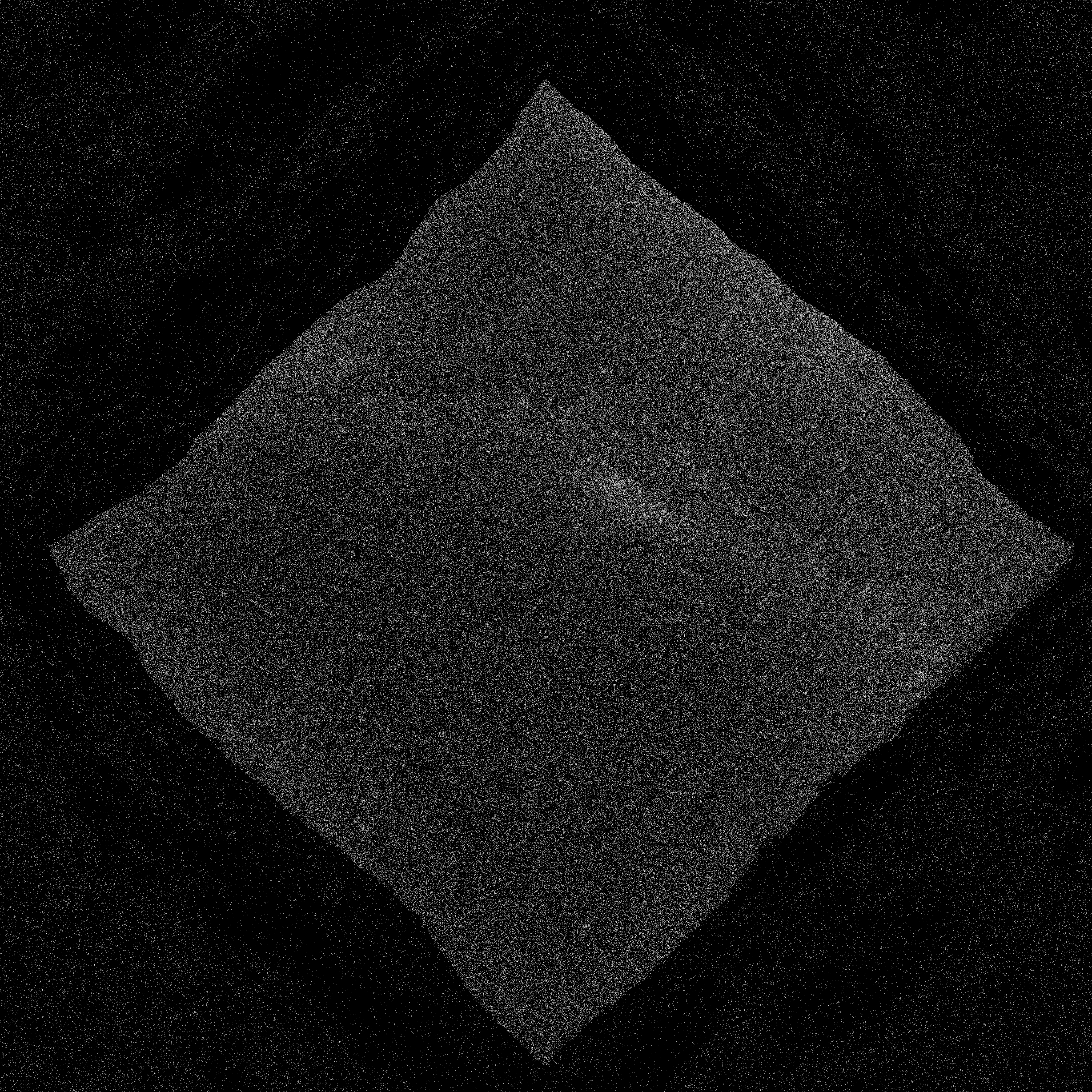
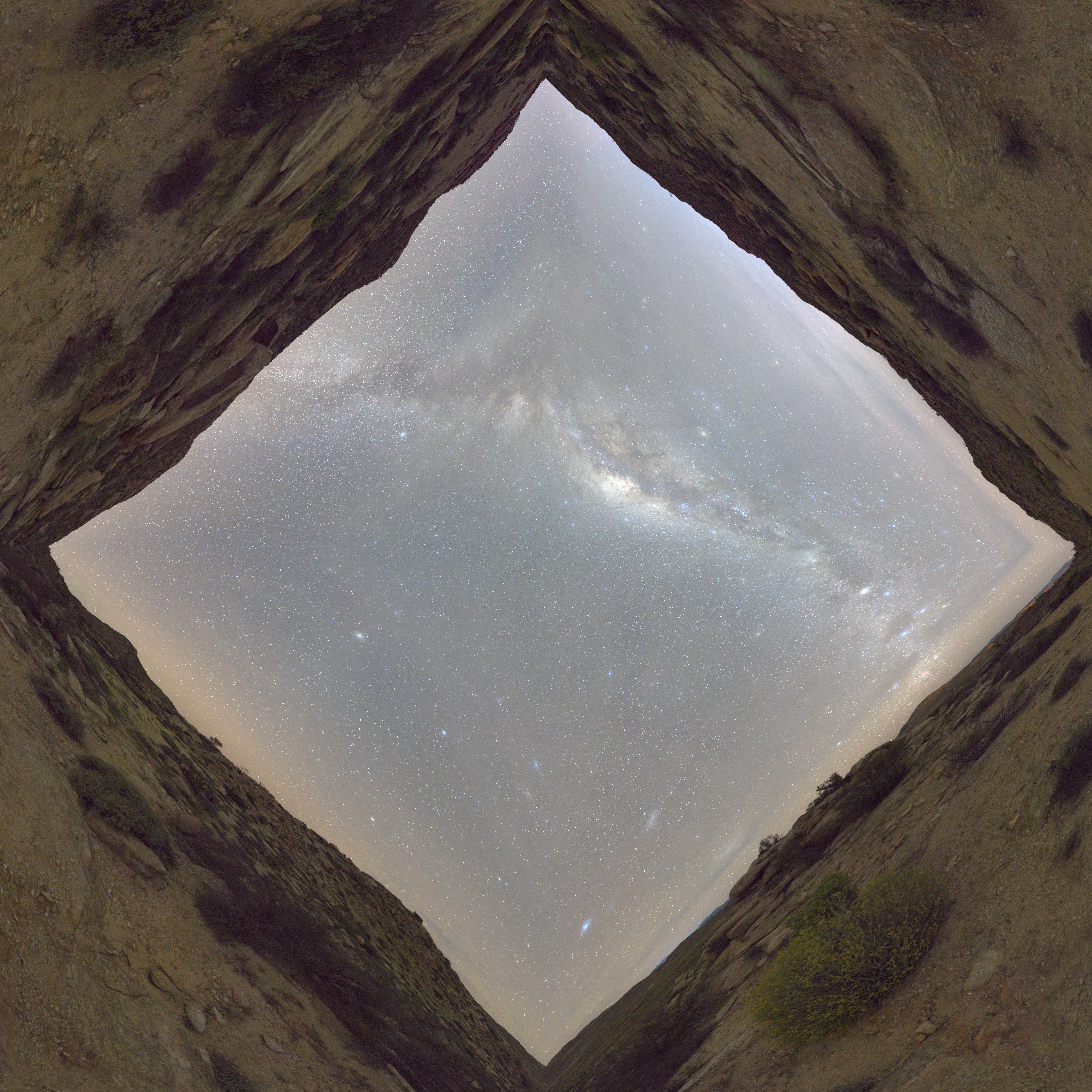
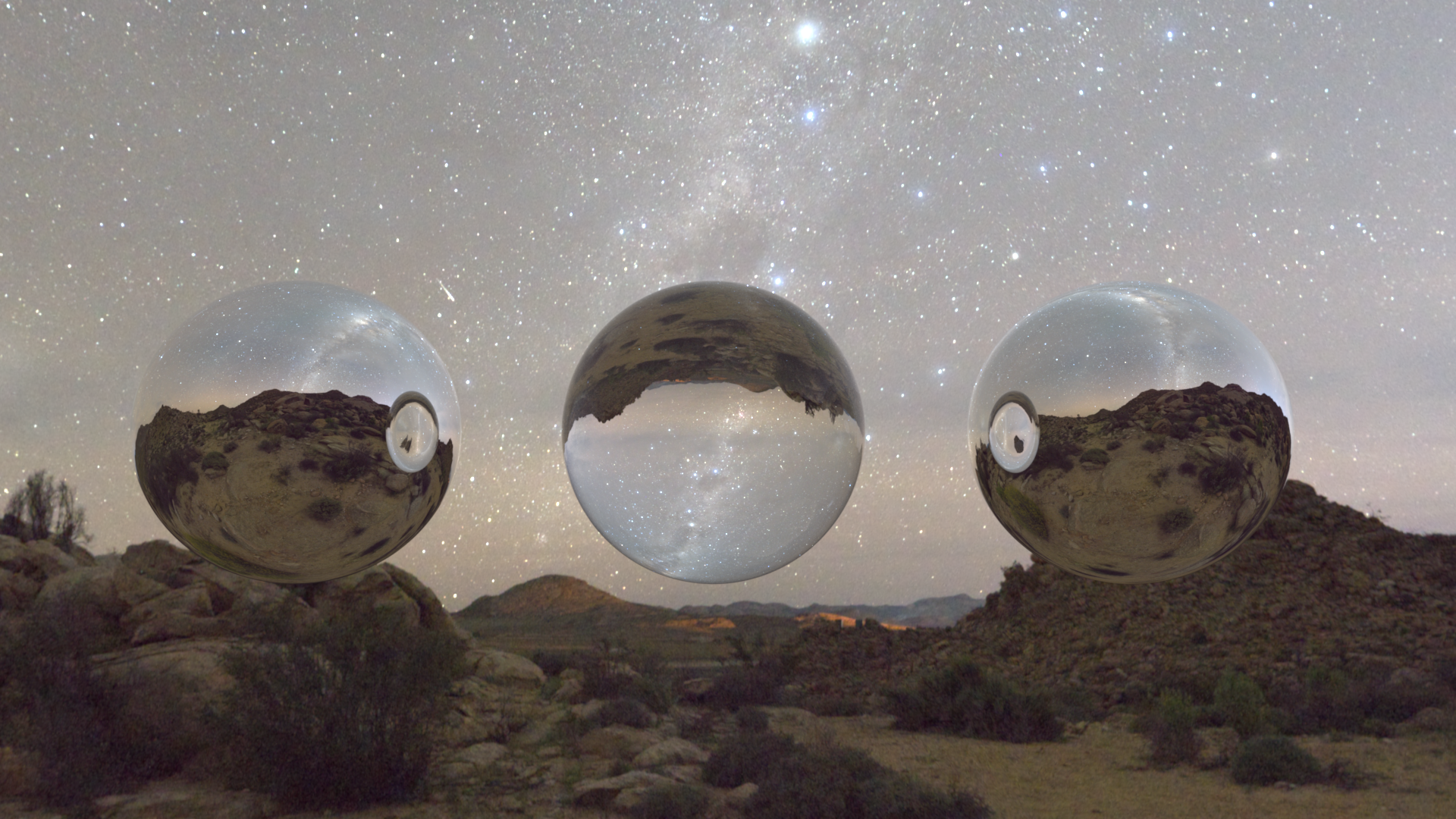
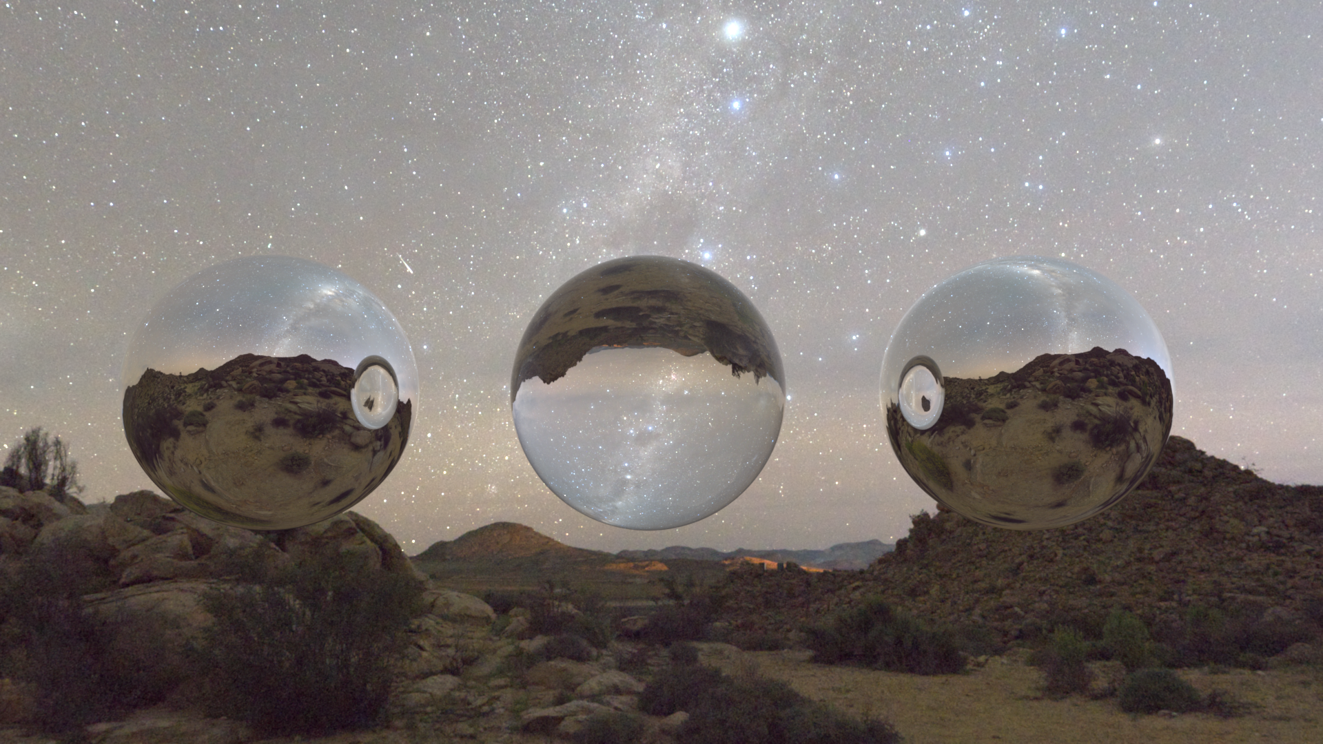
The environment used for validation here was taken from PolyHaven:
which was converted to an equal area map using latlong_to_equalarea.py. The upper hemisphere (the sky) is mapped to the centre diamond, and the lower hemisphere (the ground) is mapped to the four corners, just as described in the description above. Sampling is proportional to the luminance, as seen in the heat map below (brighter pixels represent more frequent sampling).
The validation scene against Mitsuba:
Textures ↑
Images as Texture ↑
Description ↑
Files created or modified:
include/nori/lodepng.h: downloaded from lodepngsrc/lodepng.cpp: downloaded from lodepngsrc/imagetexture.cpp
Validation scenes:
scenes/nori-beyond/image_texture/mesh-image-texture.xmlscenes/nori-beyond/image_texture/mesh-image-texture-mitsuba.xml
This feature enables the use of PNG images as textures to replace constant albedo colors on objects in the scene. A new texture type ImageTexture is implemented in imagetexture.cpp. The texture supports tiling and scaling.
The standard texture mapping pipeline includes scene definition -> texture loading at startup -> ray intersection -> UV coordinate interpolation -> texture lookup -> colour / material evaluation. To breakdown the implementation, the following details the pipeline:
- Image texture loading at startup: An image loader would be needed to parse the image file in order to handle decompressing data, convert to RGB format, etc.
- Ray intersection: When a ray hits a mesh triangle, I would need to get the barycentric coordinates of the hit point within the triangle
bary_coordinates. - UV coordinate interpolation: The 3D mesh has UV coordinates stored per vertex, normalized to . For example,
Point2f uv0 = m_UV.col(v0)is the UV coordinates at vertex 0. Usingbary_coordinates, I can interpolate the UV coordinates:its.uv = bary_coordinates.x() * uv0 + bary_coordinates.y() * uv1 + bary_coordinates.y() * uv2. This part and the previous two parts are already handled in nori. - Texture lookup: I need to loopk up the colour in the loaded texture data. This consists of first converting the UV coordinates () to pixel coordinates ([width, height]), then looking up the image loader data.
- Colour/Material evaluation: This is implemented in the BSDF
evalmethods (e.g.Diffuse'sevalmethod callsm_albedo->eval(bRec.uv)). Finally, the BSDF value is evaluated withbsdf->eval(bRec).
For the image loader, I searched for commonly used ones and were deciding between lodepng and stb_image. I decided to use lodepng since I only need PNG support and that it has separate compilation and has automatic memory management.
For the PNG image loading, I first construct the flattened 1D array m_data in which each entry is a Color3f, for memory efficiency.
ImageTexture::eval(...)
Given the UV coordinates on the 3D surface, this method should find the corresponding pixel in the image texture, and return its RGB colour.
First, apply the tiling and scaling by computing the fractional part of the scaled UV coordinates
float img_u = std::fmod(uv.x() * m_scale.x(), 1.0f);
float img_v = std::fmod(uv.y() * m_scale.y(), 1.0f);
For example, if uv = (0.75, 0.75) and m_scale = (2.0, 2.0), then after scaling, I get (1.5, 1.5) which is beyond and I are in the second repetition, so I subtract by to get , which means that at surface point I sample texture from , because the texture is repeated twice.
Next, convert the UV coordinates to pixel coordinates by scaling img_u by m_width and img_v by m_height and trancating to integer pixel index. For the V coordinate, I need to flip the axis because in the image storage, row 0 is at the top of the image but V = 0 is at the bottom of the texture. Then I clamp the bounds to prevent the pixel coordinates being negative or going beyond the last column or row.
Finally, convert from 2D to 1D array index to look up the RGB value from m_data which I constructed.
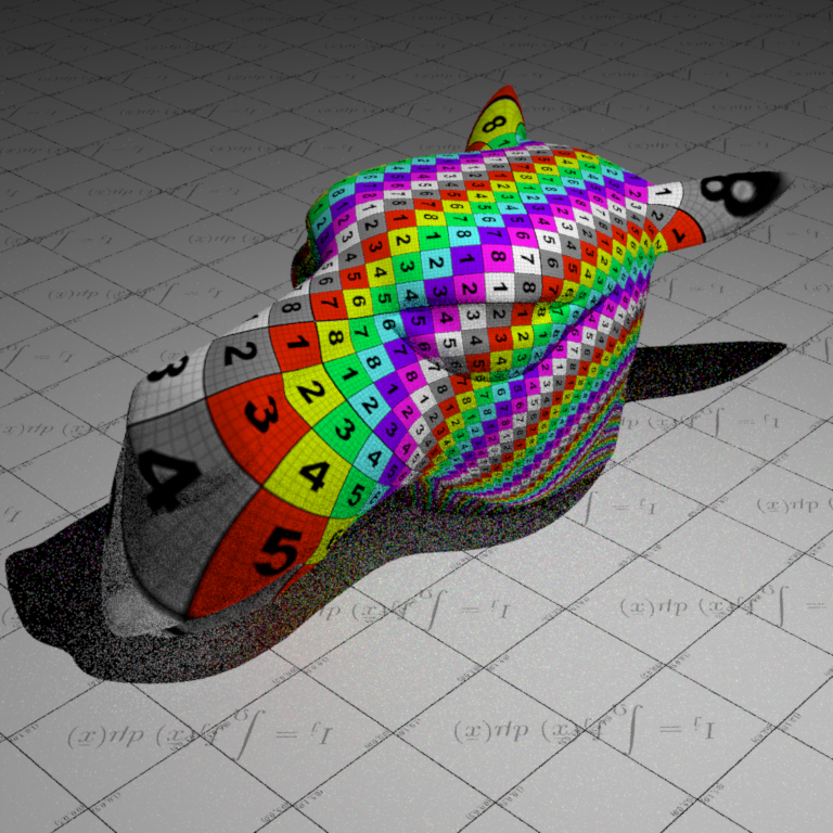
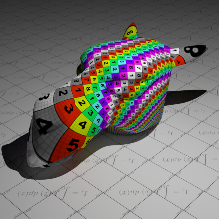
Validation ↑
For the validation scenes, I reuse the scene mesh-texture from assignment 1

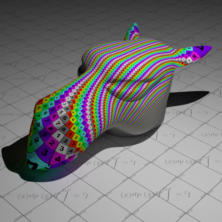
Normal mapping ↑
Normal mapping replaces the shading normal with a normal sampled from a texture (RGB image). The texture stores perturbations of the normal direction. This feature is discussed in chapter 10.5.3 of the PBR book.
Description ↑
Files created or modified:
src/normalmap.cppinclude/nori/bsdf.hsrc/diffuse.cppsrc/mesh.cpp
Validation scenes:
scenes/nori-beyond/normal_mapping/mesh-normal-map.xmlscenes/nori-beyond/normal_mapping/mesh-no-normal-map.xmlscenes/nori-beyond/normal_mapping/mesh-normal-map-mitsuba.xmlscenes/nori-beyond/normal_mapping/mesh-no-normal-map-mitsuba.xml
The current rendering pipeline follows ray generation -> ray-scene interaction -> mesh.cpp::setHitInformation which fills in its -> integrators to compute radiance. The NormalMap texture would return the Normal3f at a given UV coordinate in the 3D surface. We need to modify mesh.cpp::setHitInformation so that its.shFrame is the perturbed frame according to the normal map.
src/normalmap.cpp
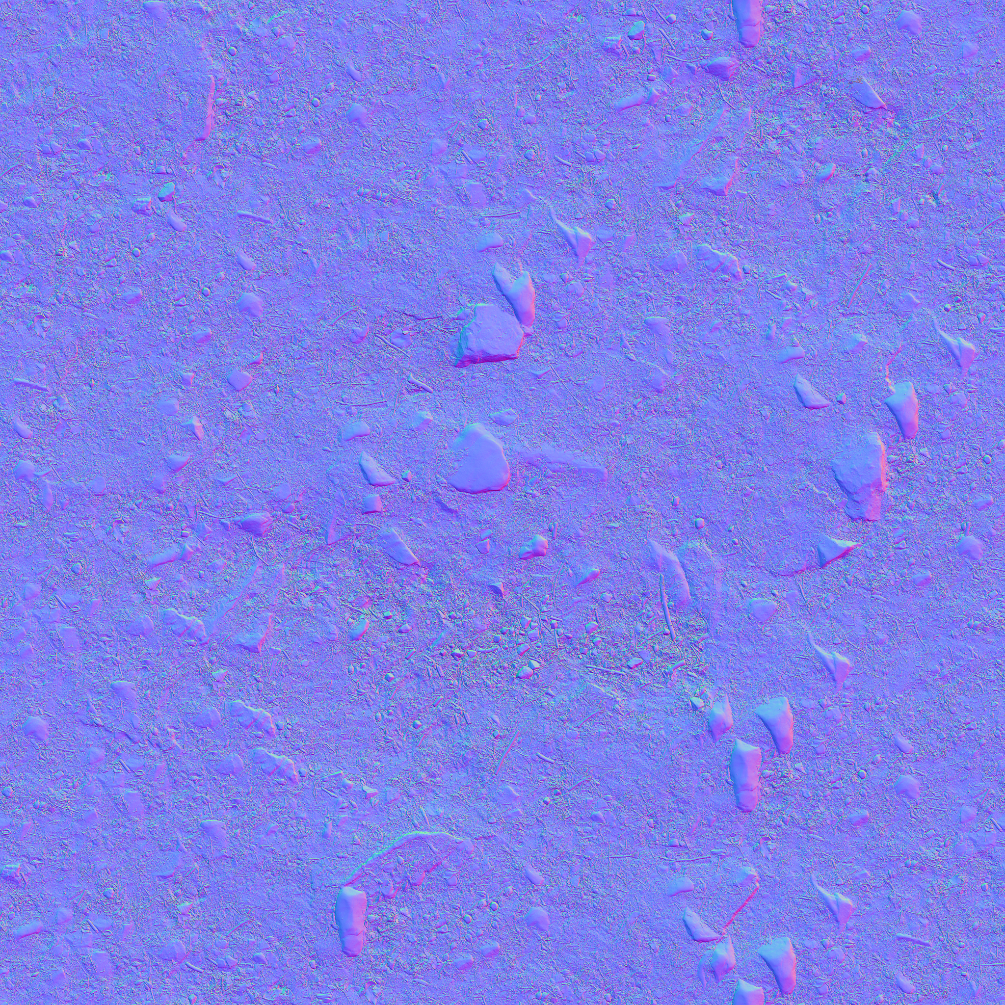
A new texture NormalMap is implemented in normalmap.cpp. Normal maps are stored in the tangent space (aligned with per-vertex tangent, bitangent, normal) using (R, G, B) = (nx, ny, nz) with each component in . Since real normals are in , the PBR book decodes them by x = 2 * r - 1, and correspondingly for y and z. After that, we store the Normal3f(x, y, z) into m_data. In include/nori/frame.h, the Frame class defines s and t as tangent vectors and n as the normal and the key transformation method is:
Vector3f toWorld(const Vector3f &v) const {
    return s * v.x() + t * v.y() + n * v.z();
}
which is a standard right-handed coordinate frame with no special tangent convention defined. So for normal maps with OpenGL format, we pass through (x, y, z) which will be mapped to (s, t, n) and for normal maps with DirectX format, we pass (x, -y, z) since DirectX conventions have Y pointing down. Other than this detail and that the final returned Normal3f should be normalized, the implementation of eval is the same as as that in ImageTexture.
include/nori/bsdf.h
We added the method getNormalMap() which returns true if the BSDF has a normal map. We need to add this method because image textures are stored in m_albedo within the BSDF (diffuse.cpp::addChild()), and then the sample method uses it. However, since we need to modify its.shFrame inside mesh.cpp::setHitInformation, it must access m_normalMap.
src/diffuse.cpp
To use the normal map, we need at least one BSDF that stores it. We use the diffuse BSDF. For each instance where m_albedo appears, we also add m_normalMap. This includes the constructor, destructor, addChild() and toString(). In addition, we also implement the getNormalMap() override to return the normal map so the mesh can retrieve it.
Mesh::setHitInformation()
After interpolating base normal from mesh, we need to query BSDF for the normal map using getNormalMap(). If normal map exists, we evaluate the normal map at its.uv to get the tangent-space normal. Then we compute the tangent frame from UV gradients and transform the normal to world space. Then we update its.shFrame with the perturbed normal. In detail, we first read the normal map using Normal3f mappedNormal = normalMap->eval(its.uv), where eval was implemented in normalmap.cpp.
Let the triangle vertex positions be and the triangle UVs be . We define , , , . We want solving the linear system coming from
Equivalently,
Solving for by inverting the UV matrix, the determinant is
If , the inverse yields the closed form
If , the UV mapping is degenerate (no well-defined mapping), so we fall back. Next we Gram-Schmidt the tangent. We set Vector3f n = its.shFrame.n;, then to compute , we project on to normal by . Then remove the normal component
and normalize it. Then compute bitangent as cross product: . Then we do a linear change-of-basis from tangent-space coordinates to world coordinates using the TBN matrix :
and normalize it. Then, we replace the shading normal used for shading with the perturbed normal . The new shading frame is constructed from .
For the fallback branch (degenerate UV) or if there is no UV, we cannot reliably compute from UV, so we use the preexisting tangent frame.
Validation ↑
The materials used for validation are downloaded from ambientCG:
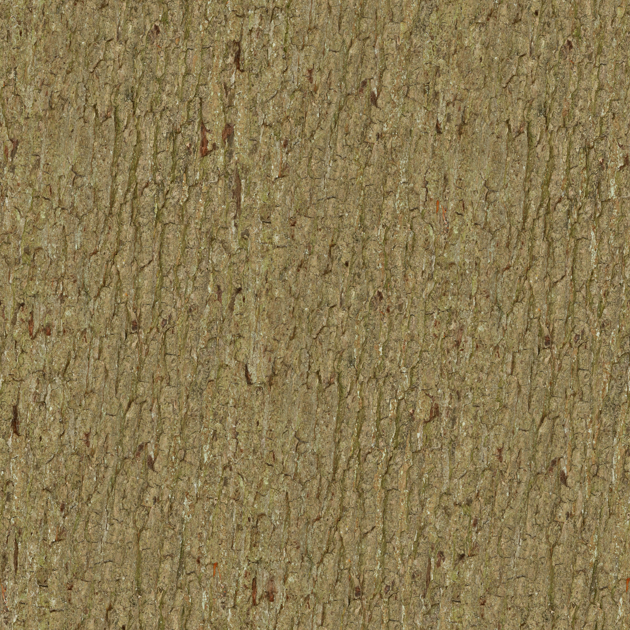
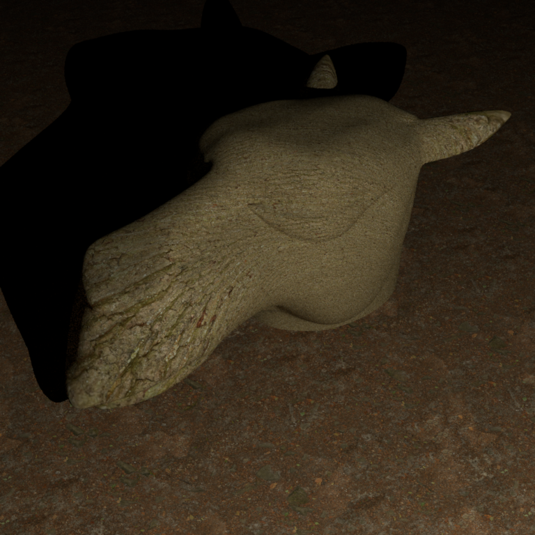
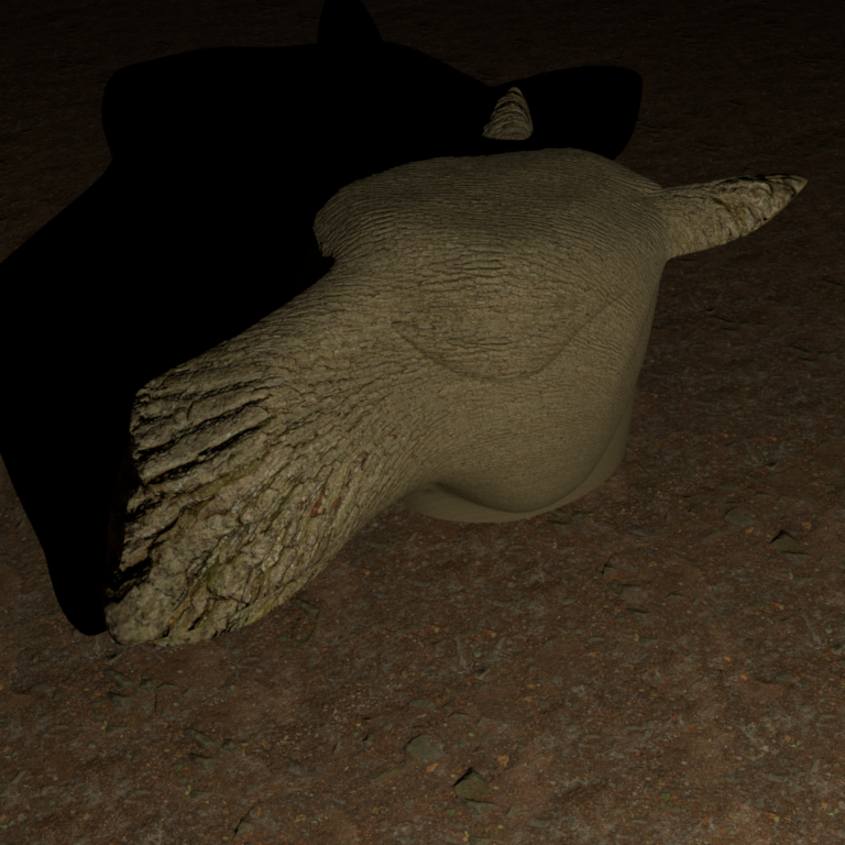
Bark Color Map
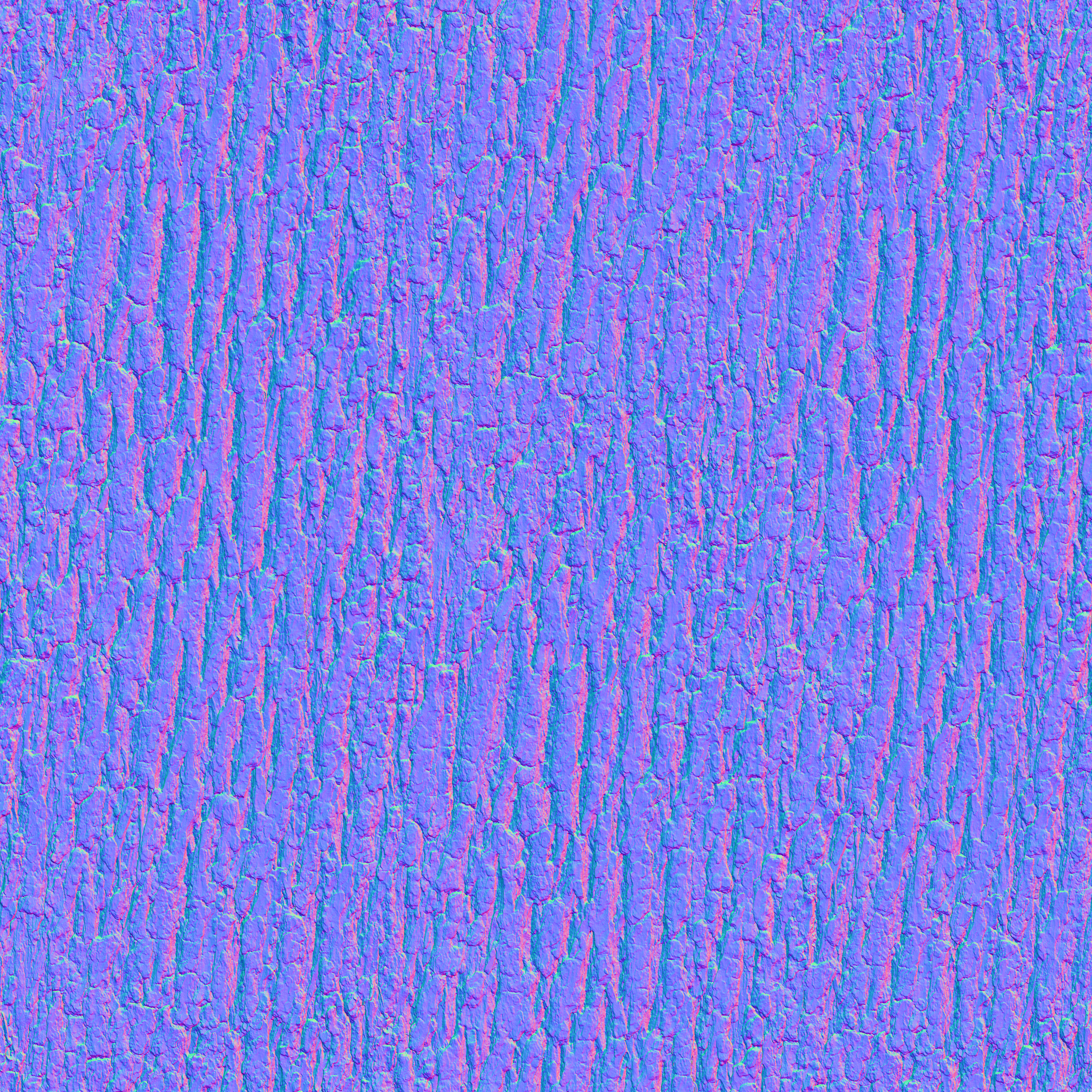
Bark Normal Map
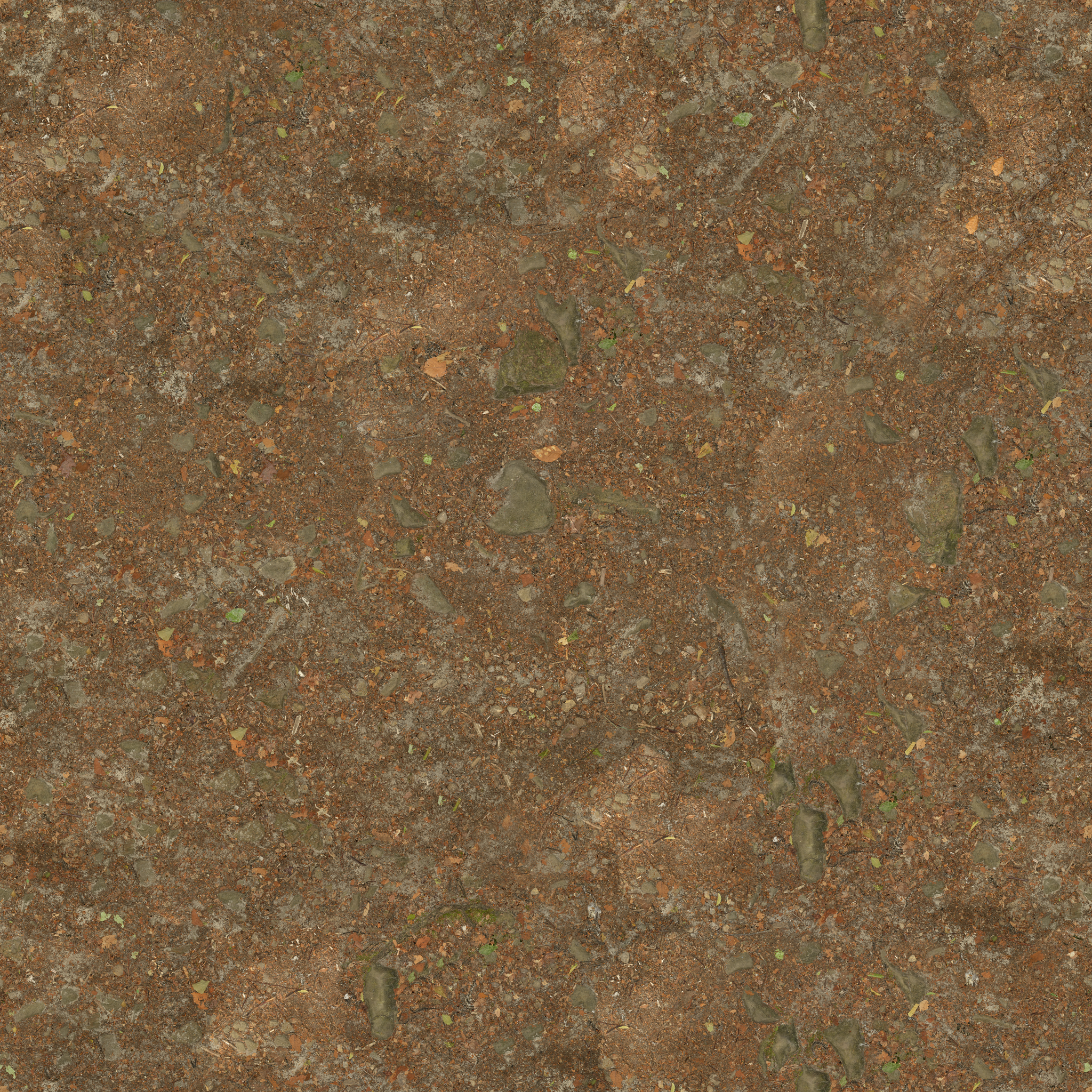
Ground Color Map
Ground Normal Map
Comparison: Bark and Ground Material With and Without Normal Maps


Light Transport Algorithms ↑
Final Gather for Photon Mapping ↑
Final Gather for Photon Mapping refines global illumination by gathering photon data to compute indirect light.
In standard photon mapping, we estimate irradiance by averaging photons within a radius . This is inherently biased because we are averaging over an area, not evaluating at a point. Sharp features get smeared. The larger the radius, the more blur, and the smaller the radius, the more noise. Final gather hides the bias behind an integration.
Description ↑
Files created or modified:
src/photonmapper.cpp
Validation scenes:
scenes/nori-beyond/final_gather/cbox_0.xmlscenes/nori-beyond/final_gather/cbox_64_10M.xml
The basic photon mapping logic has two phases: preprocessing and rendering. The preprocessing phase follows the steps:
- Emit photons from light sources until the desired number of photons stored in map
num_photonsreaches the target number of photonsm_photonCount. Randomly select an emitter, sample a photon ray and power usingsamplePhoton(). - Trace photons through the scene :
- When a photon hits a diffuse surface, store it in the photon map (position, incident direction, power)
- Use Russian roulette for path termination
- Sample BSDF to bounce the photon, attenuating its power by
- Account for radiance scaling when passing through dielectric surfaces with scaling
- Build KD-tree for efficient photon lookups
The rendering phase follows the steps:
- Trace camera rays through the scene
- If the ray hits an emitter, add emitted radiance .
- At the first diffuse surface hit,
- Search photon map within
m_photonRadius - For each found photon , evaluate BSDF (with the current ray direction and the photon direction ) and accumulate with .
- Get density estimation where is the number of emitted photons.
- Aggregate by multiplied by the current throughput
- Search photon map within
- Use Russian roulette for path termination
- At specular surfaces, continue tracing via BSDF sampling.
PhotonMapper::Li()
Instead of looking up photons at the point of query , we do one extra bounce. We sample m_numGatherRays gather rays from with its BSDF. We trace each gather ray through the scene with max maxSpecularBounces specular bounces. At the first diffuse hit, we perform the photon lookup and density estimation. The radiance , from final gather is then given by
A caveat about final gather is that we need to explicitly compute direct lighting with a shadow ray test. Consider direct photon density estimation: Without final gather, photons from the light hits surfaces and get stored. A sphere blocks photons from reaching the floor behind it. Fewer photons are then stored in that shadowed region, causing it to be darker and creating shadows. With final gather, gather rays are shot from the shading point in all directions, where we look up photons. Even if the shading point is in shadow, the gather ray can reach lit surfaces, causing the shadow to disappear. Hence the radiance at , is given by where is the throughput.
The current code now takes in an argument numGatherRays as follows:
<integrator type="photonmapper">
		<float name="photonRadius" value="0.05"/>
		<integer name="photonCount" value="10000000"/>
        <float name="numGatherRays" value="64"/>
</integrator>
If numGatherRays is unspecified, it is automatically set to 0, and the behaviour is the same as original version of photon mapping.
Validation ↑
It can be observed that the caustic effect gets diluted or lost. This is because caustic photons (light paths like ) are stored in the global photon map. Without final gather, we query photons directly at the shading point, and caustics are visible. With final gather, the gather rays sample the BSDF and do photon lookups at the endpoints of those rays. However, caustics are highly localized and the probability that a random gather ray lands exactly in a caustic region is very low, and thus most gather rays missthe caustic entirely. So the caustic effect gets diluted.

Dedicated Caustics Photon Map ↑
A dedicated caustics map separates photons into two categories: Global photon map and caustics photon map. The caustics photon map stores photons that passed through at least one specular surface before hitting a diffuse surface.
Description ↑
Files created or modified:
src/photonmapper.cpp
Validation scenes:
scenes/nori-beyond/caustics_map/cbox_64_10M.xml
New member variables m_causticPhotonCount, m_causticRadius, m_emittedCausticPhotons have been added. In general, typical photon radius in the caustics map is smaller than that in the global map, and fewer photons are needed.
PhotonMapper::preprocess()
The preprocessing phase now needs to build two photon maps. photonCount photons are to be stored in the global photon map and stored at diffuse surfaces. If caustics photon map is enabled, the photons are stored only if they did not just hit a specular surface one bounce ago. Otherwise if caustics photon map is disabled, they are stored at every diffuse hit. causticPhotonCount photons are to be stored in the caustics photon map. We track a flag hasHitSpecular, initialized as false, as the photon bounces in the scene. Once the photon has hit a specular surface, the flag is set to true. In the next diffuse hit, the photon is stored in the caustics map and we stop tracing this photon.
PhotonMapper::Li()
At a diffuse surface, we estimate the photon density from the caustics map without final gather and obtain . We also estimate the photon density with the global photon map with or without final gather (depending on user specification) and obtain . We then aggregate the two radiances.
The current code now takes in an argument causticPhotonCount and causticRadius as follows:
<integrator type="photonmapper">
    <integer name="photonCount" value="10000000"/>
    <float name="photonRadius" value="0.05"/>
    <integer name="numGatherRays" value="64"/>

    <integer name="causticPhotonCount" value="2000000"/>
    <float name="causticRadius" value="0.02"/>
</integrator>
If causticPhotonCount or causticRadius are unspecified, they are automatically set to 0, and the behaviour is the same as original version of photon mapping.
Validation ↑
Resampled Importance Sampling ↑
Resampled Importance Sampling (RIS) focuses computation on areas of higher light contribution.
In the current path tracing with multiple importance sampling (MIS), we sample one light uniformly from the light set, and one BSDF direction, and combine the two with MIS weights. This works well, but uniform light selection is bad when many lights exist, and one light sample per bounce is often noisy. In RIS, we generate candidate lights, assign each a weight, and resample one candidate. When , RIS reduces to standard emitter sampling.
Description ↑
Files created or modified:
src/path_ris.cpp
Validation scenes:
scenes/nori-beyond/path_ris/sponza.xml
The general RIS framework from Talbot et al. estimates an integral using two PDFs:
- Source PDF : easy to sample from (the proposal distribution)
- Target PDF : closer to , possibly unnormalized or difficult to sample directly
The RIS procedure is:
- Draw candidate samples
- Compute resampling weights
- Resample one candidate from with probability
- The unbiased RIS estimator is:
When , RIS reduces to standard importance sampling with PDF .
Our implementation uses a simplified parameterization where we set (the target equals the integrand). This is a valid special case of RIS.
For direct lighting at shading point , the integrand is:
where is a point on a light source, , is the geometry term, and is visibility.
Our source (proposal) PDF is uniform light selection combined with area sampling on each light:
with .
PathRISIntegrator::Li()
At shading point :
-
Sample candidates. For , sample light uniformly such that , and sample point on light :
-
For each candidate, compute the contribution (ignoring visibility for now):
Note that is the integrand divided by the solid angle PDF only (not the full proposal PDF). The factor is handled separately. Also compute the scalar resampling weight .
-
Select candidate with probability
-
If the selected candidate passes the visibility test, compute the final estimate. When (our case), , so the estimator simplifies to . However, computing the full sum requires evaluating all candidates. In practice, we select candidate with probability , then output . By importance sampling, this has the same expectation as the full sum but only requires evaluating one candidate (e.g., one visibility test instead of ). Using the this single-sample RIS variant with , the estimator is:
But this assumes with the full proposal PDF . In our implementation, we instead use where (missing the factor). To correct for this, we multiply by :
The term gives us the correct importance sampling ratio for the full proposal PDF.
When , , recovering standard emitter sampling: .
For the emitter sampling branch (RIS), we apply a MIS weight:
where is the full emitter sampling PDF (solid angle PDF divided by number of lights) and is the BSDF sampling PDF. The final RIS contribution becomes:
For the BSDF sampling branch, when a BSDF-sampled direction hits an emitter, we apply the complementary MIS weight:
and add:
For delta BSDFs (mirrors, glass), is a Dirac delta and emitter sampling cannot find specular paths, so we use for BSDF-sampled paths through specular surfaces.
Validation ↑
This Sponza scene features multiple area lights distributed throughout the space, creating complex lighting conditions where uniform light selection becomes inefficient. Many shading points receive significant contribution from only a subset of the lights (e.g., nearby lights or those with unobstructed paths), while distant or occluded lights contribute little.
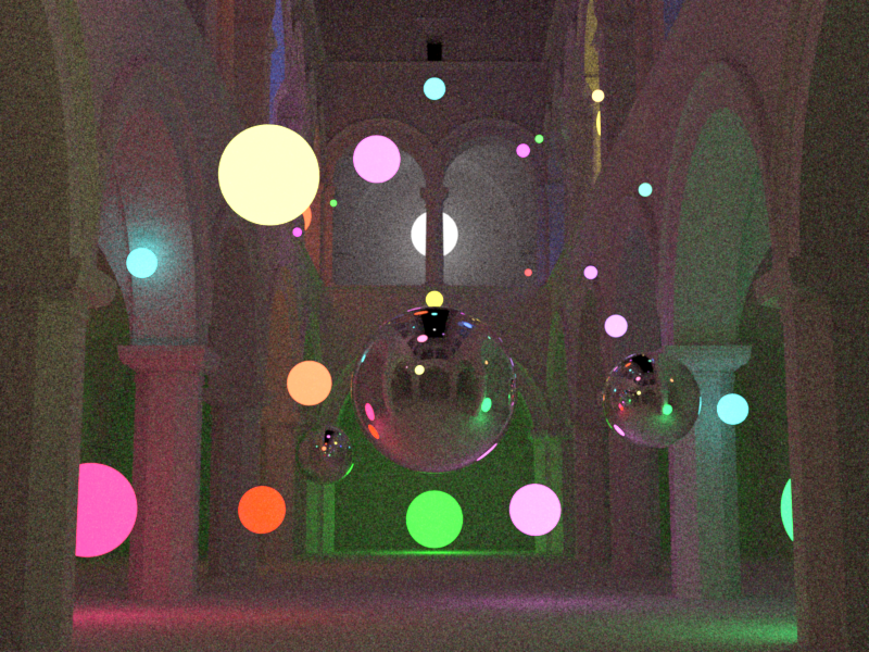
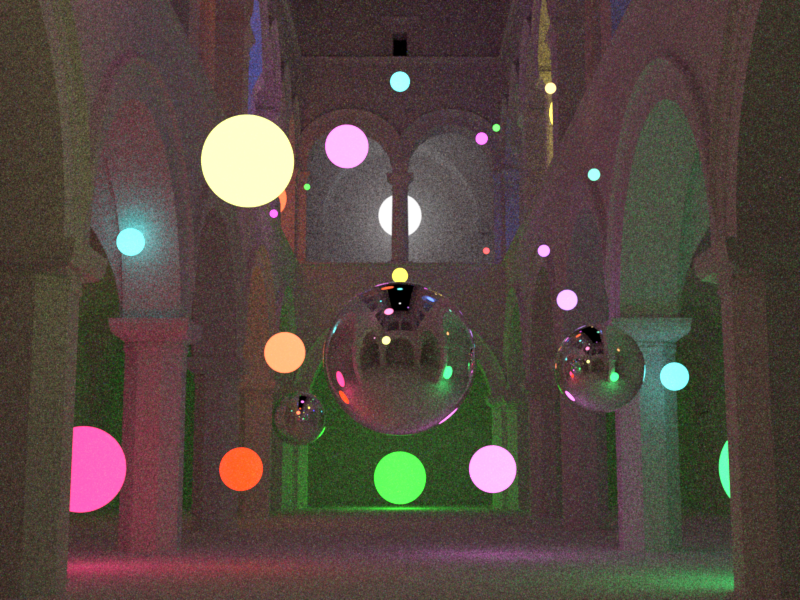
RIS excels in this scenario by resampling candidates based on their actual contribution (BSDF emission geometry), effectively concentrating samples on the lights that matter most for each shading point. This leads to lower variance compared to MIS with uniform light selection at the same sample count.
Participating Media ↑
Phase Functions ↑
The phase function describes the angular distribution of light as it is scattered at a point within a medium. It is the volumetric analog of the BRDF for surfaces. Unlike a BRDF, which is normalized by a cosine factor and can integrate to values less than 1 (due to absorption), a phase function represents a pure probability density function (PDF) over the sphere of directions. Therefore, it must integrate to unity:
Description ↑
The phase functions implemented are the isotropic phase function and the henyey-greenstein phase function.
In isotropic scattering, light is scattered equally in all directions. This is the volumetric equivalent of a perfectly diffuse Lambertian surface. Since there are steradians in a unit sphere,
In many real-world media (like clouds or smoke), scattering is highly anisotropic, meaning it favors certain directions. Henyey-Greenstein is a popular empirical model used to simulate this behavior:
where is the angle between the incoming and outgoing directions. The parameter (the asymmetry parameter or mean cosine) defines the "shape" of the scattering:
- : Forward scattering (light continues mostly in the same direction).
- : Backscattering (light is reflected back toward the source).
- : Isotropic scattering (mathematically equivalent to the isotropic model).
The value of is defined as the average cosine of the scattering angle:
where . For example, if , the "average" photon is deflected only () from its original path.
Files created or modified:
include/nori/phasefunction.hsrc/isotropic.cppsrc/henyey_greenstein.cpp
Validation scenes:
include/nori/phasefunction.h
This file mirrors the BSDF interface for consistency. It includes a PhaseFunctionQueryRecord, similar to the BSDFQueryRecord, and supports two constructors of a PhaseFunctionQueryRecord -- one that takes in the incident direction for sampling the outgoing direction , and one that takes in both and for evaluation.
The PhaseFunction object is the superclass of all phase functions and has the methods sample and eval. Unlike BSDF which also has the pdf method, phase functions are PDFs themselves, hence eval will return the phase function value (i.e. the PDF). The sample method in PhaseFunction also returns the phase function value for convenience (instead of 1.0, which would be case in the BSDF implementation that returns eval() / pdf()).
Isotropic::sample(...)
Given a sample , we sample a direction uniformly on a sphere with Warp::squareToUniformSphere and assign this direction to pRec.wo. The method returns the phase function value is .
Isotropic::eval(...)
The phase function value is simply for any given pairs of and .
HenyeyGreensteinPhaseFunction::sample(...)
The azimuthal angle is simply since Henyey-Greenstein does not depend on it. For the polar angle, we need to find by inverting the CDF. The marginal PDF for is obtained by integrating over :
The CDF is obtained by integrating from to . Let , so :
Setting and solving for :
Squaring both sides and solving for :
For the special case (isotropic), we use uniform sphere sampling: .
Once and are computed, we build a coordinate frame around the forward scattering direction and convert from spherical to Cartesian coordinates to obtain .
HenyeyGreensteinPhaseFunction::eval(...)
The method simply computes for the given pair of and , and returns
Validation ↑
Transmittance in Homogeneous Media ↑
This feature enables coloured dielectric materials and fog volumes using Beer's law transmittance for homogeneous participating media.
Description ↑
By Beer's law, in a homogeneous participating medium (where the absorption coefficient is constant), the transmittance of light is given by
where is the distance travelled.
Files created or modified:
include/nori/bsdf.hsrc/null.cppsrc/dielectric.cppsrc/path_mis.cpp
Validation scenes:
scenes/nori-beyond/homogeneous_media/cbox_colored_glass.xmlscenes/nori-beyond/homogeneous_media/cbox_colored_glass_mitsuba.xml
include/nori/bsdf.h
The BSDF interface is extended to include absorption with default no-absorption behaviour. New virtual methods getAbsorptionCoefficient() (returns Color3f(0.0f) by default) and hasAbsorption() (returns false by default) are added. A method isNull() (returns false by default) is also added to distinguish null/transparent surfaces from real surfaces during ray marching.
src/null.cpp
This is a null/transparent BSDF that lets rays pass through without any scattering or reflection. It is used to bound fog volumes without any refractive distortion. It overrides hasAbsorption and getAbsorptionCoefficient to expose the volume's absorption coefficient, and isNull to return true. The null BSDF has discrete measure and returns zero for eval and pdf. In the sample method, it sets to (ray passes straight through) and to 1 (no index of refraction change). It can be used in the scene like this:
<mesh type="obj">
    <string name="filename" value="fog_box.obj"/>
    <bsdf type="null">
        <color name="sigmaA" value="0.5, 0.5, 0.5"/>
    </bsdf>
</mesh>
src/dielectric.cpp
The dielectric BSDF is extended with a new Color3f member variable m_sigmaA, which stores the absorption coefficient per RGB channel. The methods getAbsorptionCoefficient and hasAbsorption are overridden. The absorption itself is not applied by the BSDF; it is handled by the integrator via Beer's law on each ray segment inside the medium.
PathMISIntegrator::Li(...)
The integrator uses a medium stack (std::vector``<``const BSDF *>) to track which absorbing volumes the ray is currently inside. This stack-based approach correctly handles arbitrarily nested media (e.g. a coloured glass sphere inside a fog cube). The innermost medium on the stack determines the active absorption coefficient.
The core procedure is null-surface marching: given a ray, we step through all null (transparent) boundaries until we reach a real surface, applying Beer's law and updating the medium stack at each step. This procedure is used in three contexts:
- Initial ray marching (camera ray to first real surface)
- Shadow rays (emitter sampling, using a separate copy of the medium stack)
- BSDF-sampled rays (path continuation after bouncing off a real surface)
The null-surface marching procedure works as follows:
- Trace the ray to the nearest surface intersection.
- Look up the current absorption coefficient from the top of the medium stack (zero if the stack is empty).
- Apply Beer's law: multiply the throughput by , where is the distance to the intersection.
- If the intersected surface is not null (i.e. it is a real surface like a diffuse wall or dielectric), stop marching and return this intersection.
- Otherwise, the surface is null (a medium boundary). Update the medium stack:
- If the ray is entering the volume (ray direction dot geometric normal ), push the null surface's BSDF onto the stack.
- If the ray is exiting the volume (ray direction dot geometric normal ), find and remove this BSDF from the stack.
- Advance the ray origin to the intersection point and go back to step 1.
For shadow rays, the procedure is identical except that it uses a separate copy of the medium stack (so it does not disturb the main path state), accumulates transmittance into a separate variable, and terminates early if a non-null surface is hit (the light is occluded).
For dielectric surfaces, the medium stack is updated when the BSDF samples a transmission (refraction) event. This is detected by checking whether and are on opposite sides of the geometric normal. If so, the ray has crossed the interface and the dielectric's absorption medium is pushed onto or removed from the stack.
The medium stack uses id-based removal: when exiting a volume, the stack is searched from the back (innermost) to find and remove the matching BSDF pointer. This is necessary because overlapping volumes do not always nest cleanly. In the validation scene below, the sphere straddles the fog cube boundary (it pokes above the fog). Consider a ray traveling downward through the top of the sphere into the fog:
- Ray enters the sphere (above the fog) stack:
[sphere] - Ray enters the fog cube (partway through the sphere) stack:
[sphere, fog] - Ray exits the sphere (still inside the fog) need to remove
sphere, butfogis on top
At step 3, a naive stack pop would remove fog instead of sphere, which is wrong. Searching from the back by BSDF identity correctly finds and removes sphere from below fog, leaving the stack as [fog].
Validation ↑
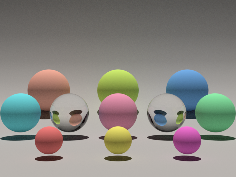
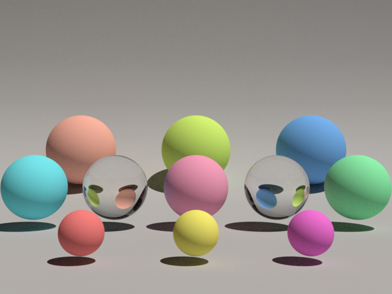
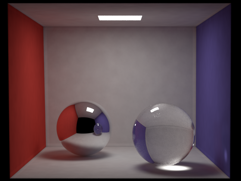
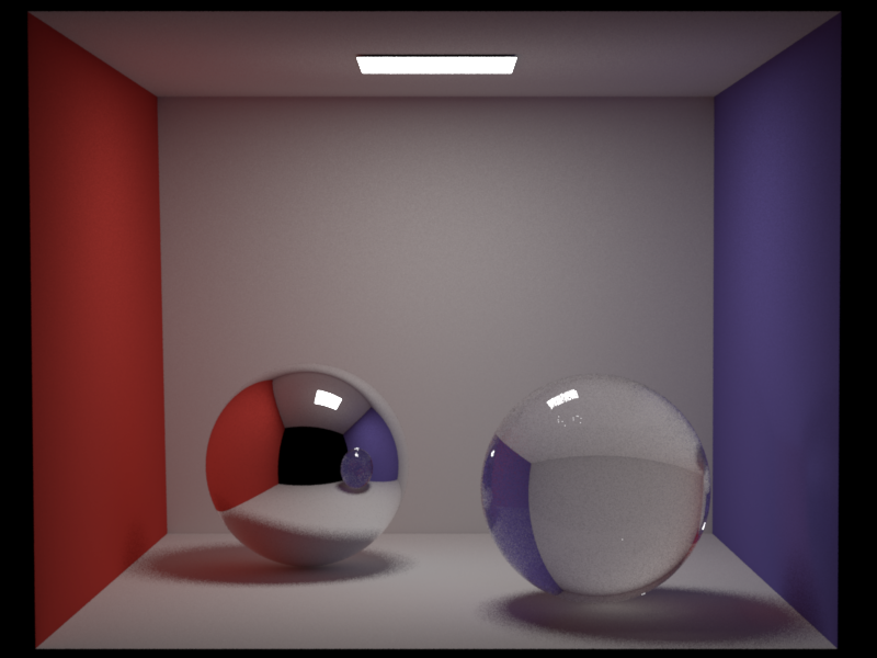
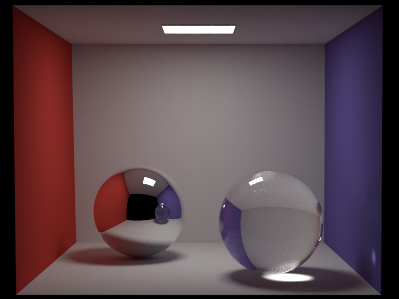
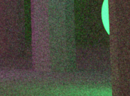
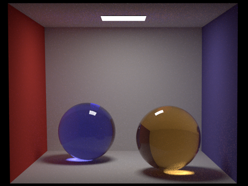
The validation scene places a blue glass sphere (null BSDF, ) and an amber glass sphere (dielectric BSDF, ) inside a fog cube (null BSDF, ) in a Cornell box. The fog cube extends through the bottom part of the room, while the spheres poke above the fog, so the fog boundary crosses each sphere near its equator.
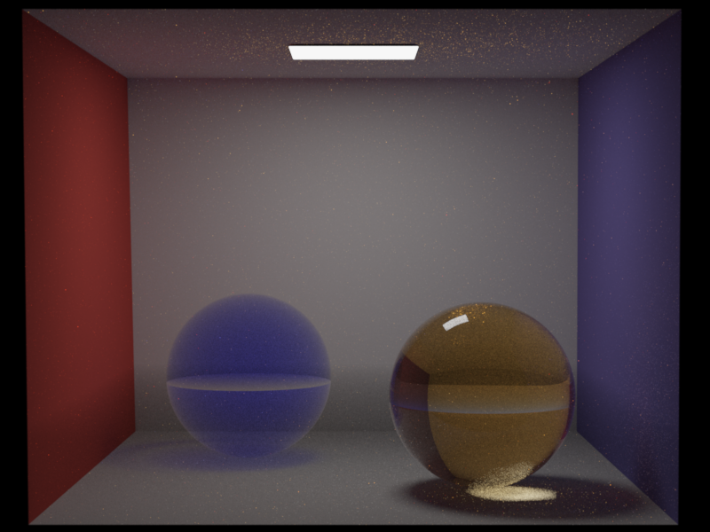
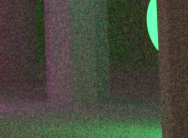
The Nori and Mitsuba renders differ due to a fundamental difference in how the two renderers track media. Mitsuba 3 uses a single medium pointer per ray: at each surface crossing, the active medium is replaced with the surface's interior or exterior medium. This produces two visible artifacts in the Mitsuba renders:
-
A visible horizontal plane across the spheres at the fog cube boundary. This appears as a brightness discontinuity where the fog cube's top face intersects the spheres. Because Mitsuba's medium pointer switches discretely at the null boundary, there is an abrupt transition between "fog active" (below the plane) and "no fog" (above the plane). In Nori, the stack-based approach produces a smooth transition because entering/exiting the fog and sphere are tracked independently.
-
A bright ring at the sphere-fog boundary in the original Mitsuba render (center image). When a ray exits the sphere (still geometrically inside the fog cube), Mitsuba sets the medium to the sphere's exterior medium. If no exterior medium is specified on the sphere, Mitsuba treats the region as vacuum, losing the fog absorption for the remainder of the segment. Rays grazing the sphere edge barely enter the sphere (little sphere absorption) and also miss the fog behind it (medium reset to vacuum on exit), producing the bright ring.
Nori uses a stack-based approach: entering a volume pushes its BSDF onto the stack, and exiting pops it. When a ray exits the sphere, the fog is still on the stack, so fog absorption continues to be applied correctly. This produces a smoother, physically correct result without the horizontal plane artifact or the bright ring (left image).
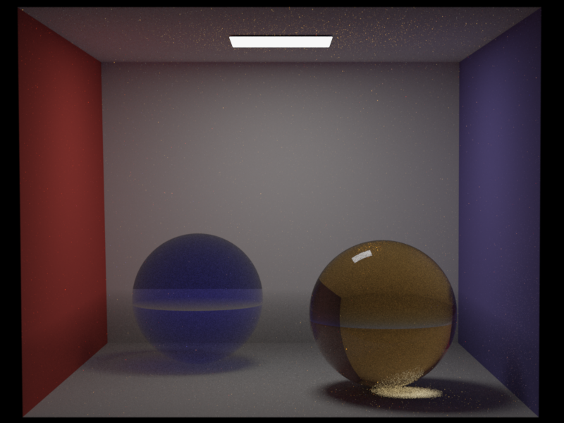
To verify this, I re-rendered the Mitsuba scene with <ref id="fog_medium" name="exterior"/> added to both spheres, which tells Mitsuba to restore the fog medium on sphere exit (right image). This largely eliminates the bright ring artifact and brings Mitsuba closer to Nori's output. However, Mitsuba's single-pointer approach still cannot fully represent the overlapping geometry: the sphere's exterior medium is set to fog everywhere, including the upper hemisphere that is above the fog cube. This means Mitsuba now over-attenuates above the fog boundary while correctly attenuating below it. Nori's stack naturally handles this because it tracks all volume boundaries the ray has crossed, regardless of the order.